The Ziggurat Algorithm for Random Gaussian Sampling

ZigguratGaussian.cs (C# source code)

The Ziggurat Algorithm is a method for efficient random sampling from a probability distribution such as the Gaussian distribution. The probability distribution function (pdf) for the Gaussian distribution is given by:

$$ y = \frac{1}{ \sqrt{(2 \pi \sigma^2}} \, e^{-\frac{(x-\mu^2)}{2 \sigma^2}} $$

Where μ is the distribution mean and σ is the standard deviation.

Internally the sampling algorithm uses a simplified pdf by using a mean of 0 and a standard deviation (sd) of 1, which allows those terms to be factored out of the the pdf. Sampling from a distribution with a different mean and/or sd is then a trivial manipulation of the generated values. The pdf is also simplified further by denormalising (factoring out constant terms) See Optimisations #2 (below).

The Ziggurat algorithm is a hybrid method that obtains its efficiency principally by using rejection sampling with some less efficient calculations performed for less commonly executed corner cases.

Rejection Sampling

Rejection sampling is a method by which uniformly distributed random samples are selected or rejected such that the selected samples have a particular desired distribution. For example in the case of a Gaussian pdf we could define a rectangular area over the main body of the Gaussian pdf (ignoring the distribution tails for a moment) and randomly generate (x,y) points within the square. We now reject all points that are above the pdf curve, i.e. where y > f(x). We can then yield the x coordinate of each of the accepted points to generate random Gaussian numbers. It is easy to see that the proportion with which points with a specific x coordinate are accepted is proportional to f(x) and therefore uniformly generated x coordinates are filtered to yield Gaussian distributed values.

Ziggurat Algorithm

The naive rejection method described above has two main sources of inefficiency.

A large proportion of samples will be rejected.
We must evaluate f(x) for each candidate point, which for many pdfs is computationally expensive.

The Ziggurat algorithm addresses these two issues by covering the pdf with a series of horizontal rectangles rather than a single square, and in an arrangement that attempts to cover the pdf as efficiently as possible, i.e with minimum area outside of the pdf curve. The following diagram demonstrates the approach. Note that we operate on one side of the pdf (x >= 0), generating both positive and negative sample values requires that that as a final step we randomly flip the sign of the generated non-negative values.

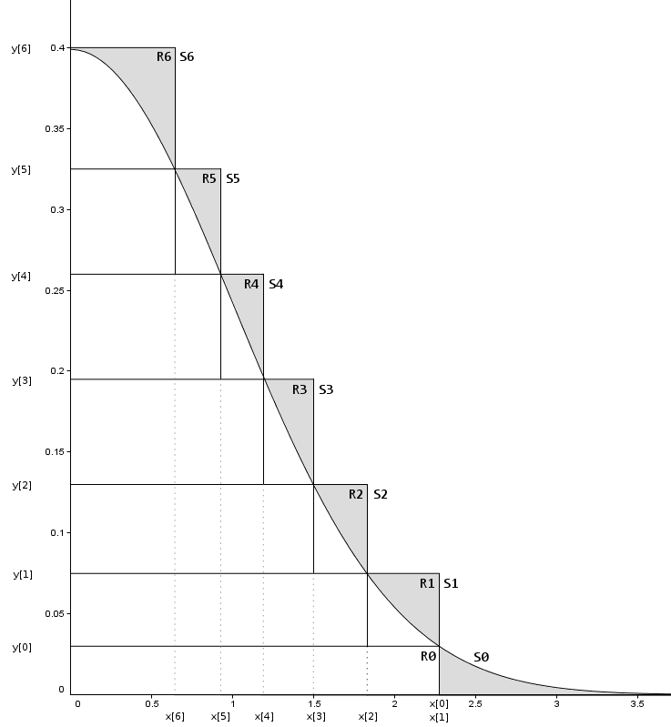
Figure 1.

Notes on Figure 1.

Each rectangle is assigned a number (the R numbers shown above).

The right hand edge of each rectangle is placed so that it just covers the distribution, that is, the bottom right corner is on the curve, and therefore some of the area in the top right of the rectangle is outside of the distribution (points with y > f(x)). However R0 is an exception and is entirely within the pdf (see next point).

R0 is a special case. The tail of the Gaussian effectively projects into x=Infinity asymptotically approaching zero, thus we do not cover the tail with a rectangle. Instead we define an x cut-off coordinate. R0's right hand edge is at the cut-off point with its top right corner on the distribution curve. The tail is then defined as that part of the distribution with x > tailCutOff and is combined with R0 to form segment S0. Note that the whole of R0 is within the distribution, unlike the other rectangles.

Segments. Each rectangle is also referred to as a segment, with the exception of R0 which is a special case as explained above. Essentially S[i] == R[i], except for S[0] == R[0] + tail.

Each segment has identical area A, this also applies to the special segment S0, thus the area of R0 is A minus the area represented by the tail. For all other segments the segment area is the same as the rectangle area.

R[i] has right hand edge x[i]. And from the diagram it is clear that the region of R[i] to the left of x[i+1] is entirely within the distribution curve, whereas the region greater than x[i+1] is partially above the distribution curve. Again noting that R0 is an exception.

R[i] has top edge of y[i].

Implementations of the algorithm typically use 128 or 256 rectangles (A) because generating values with a range that is a power of 2 is computationally efficient, and (B) because a greater number of rectangles covers the pdf more efficiently (less area outside of the pdf) than a lesser number, although there will of course be an optimum number dependent on a range of factors.

Figure 1. is for demonstration purposes only and is not an accurate rendition of a valid setup, specifically the areas of the segments and rectangles are not all equal as they should be and thus their boundaries do not meet the strict criteria described in these notes.

Operation

Randomly select a segment to sample from, call this S[i], this amounts to a low resolution random y coordinate. The segments have equal area therefore we can select from them with equal probability, this is a key part of the algorithm (See special notes below).

Segment 0 is a special case. If S0 is selected then generate a random area value w between 0 and area A. If w is less than or equal to the area of R0 then we are sampling a point from within R0 (step 2A), otherwise we are sampling from the tail (step 2B).

2A - Sampling from R0. R0 is entirely within the distribution curve and we have already generated a random area value w. Convert w to an x value that we can return by dividing w by the height of R0 (y[0]).

2B - Sampling from the tail. To sample from the tail we fall back to a relatively expensive calculation using logarithms, see Generating a Variable from the Tail of the Normal Distribution, George Marsaglia (1963). Typically the cut-off x coodinate that defines the tail is chosen such that the area represented by the tail is relatively small and therefore this execution pathway is avoided for a significant proportion of samples generated.

Sampling from all other rectangles/segments other then R0/S0. Randomly select x from within R[i]. If x is less than x[i+1] then x is within the curve, return x.

If x is greater than or equal to x[i+1] then generate a random y variable from within R[i] (this amounts to producing a high resolution y coordinate, a refinement of the low resolution y coord we effectively produced by selecting a rectangle/segment).

If y < f(x) then return x, otherwise we reject the sample point and return to step 1. We specifically do *not* re-attempt to sample from R[i] (see special notes 1).

Finally, all of the above describes sampling from the positive half of the distribution (x >= 0) hence to obtain a symetrical distribution we need one more random bit to determine whether to flip the sign of the returned x value.

Special Notes

Segments have equal area and are thus selected with equal probability. However, the area under the distribution curve covered by each segment/rectangle differs due to the varying shape of the pdf where the rectangles overlap its edge. Thus it could be suggested that to avoid sampling bias that the segments should be selected with a probability that reflects the area of the distribution curve they cover not their total area, this is an incorrect approach for the algorithm as described above. To explain why consider an extreme case...

Say that rectangle R1 covers an area entirely within the distribution curve, now consider that R2 covers an area only 10% within the curve. Both rectangles are chosen with equal probability, thus the argument is that R2 will be 10x overrepresented (will generate sample points as often as R1 despite covering a much smaller proportion of the area under the distribution curve). In reality sample points within R2 will be rejected 90% of the time and we do not attempt to re-sample from R2 to obtain a an accepted sample point, instead we return to step 1 (select a segment to sample from).

If instead we re-attempted sampling from R2 until a valid point was found then R2 would indeed become over-represented, hence we do not do this and the algorithm therefore does not exhibit any such bias.

George Marsaglia's original implementation used a single random number (32bit unsigned integer) for both selecting the segment and producing the x coordinate with the chosen segment. The segment index was taken from the the least significant bits (so the least significant 7 bits if using 128 segments). This effectively created a perculair type of bias in which all x coords produced within a given segment would have an identical least significant 7 bits, albeit prior to casting to a floating point value. The bias is perhaps small especially in comparison to the performance gain (one less call to the RNG). This bias can be avoided by simply not re-using random bits in such a way. For more details on this subject see An Improved Ziggurat Method to Generate Normal Random Samples, Jurgen A Doornik

Optimisations

On selecting a segment/rectangle we generate a random x value within the range of the rectangle (or the range of the area of S0), this requires multiplying a random number with range [0,1] to the requried x range before performing the first test for x being within the 'certain' left-hand side of the rectangle. We can avoid this multiplication and indeed conversion of a random integer into a float with range [0,1], thus allowing the first comparison to be performed using integer arithmetic. Instead of using the x coord of R[n]+1 to test whether a randomly generated point within R[n] is within the 'certain' left hand side part of the distribution, we precalculate the probability of a random x coord being within the safe part for each rectangle. Furthermore we store this probability as a UInt with range [0, 0xffffffff] thus allowing direct comparison with randomly generated UInts from the RNG, this allows the comparison to be performed using integer arithmetic. If the test succeeds then we can continue to convert the random value into an appropriate x sample value.

The Gaussian pdf contains terms for distribution mean and standard deviation. We can remove all excess terms and denormalise the function to obtain a simpler equation with the same shape. This simplified equation is no longer a pdf as the total area under the curve is no loner 1.0 (a key property of pdfs), however as it has the same overall shape it remains suitable for sampling from a Gaussian using rejection methods such as the Ziggurat algorithm (it's the shape of the curve that matters, not the absolute area under the curve).

$$ y = e^{-\frac{x^2}{2}} $$

Simplified and denormalised version of the Gaussian pdf with mean = 0 and s.d. = 1.

Performance Measurements

Method	Speed (million samples/sec)	Speedup Factor (relative to Box-Muller)
Box-Muller	92.1	1.0x
Ziggurat	185.9	2.02x

Notes

The above performance benchmarks are based on generation of double precision floating point values; the equivalent benchmark figures for single precision values were similar (on the target platform - details below)

The Box-Muller method inherently produces two samples per iteration, therefore if a single sample is required then one sample must be discarded on each call, thus halving the average speed. To achieve a fair comparison between the two methods (Ziggurat vs Box-Muller), the above benchmark figures are based on population of arrays with gaussian samples, with the Box-Muller code populating two array elements per loop to fully utilise the two generated values.

Performance test platform/environment details

CPU: AMD Ryzen PRO 5750G (TSMC 7nm FinFET).
RAM: DDR4-3200, Dual Channel.
Tests are for single thread performance only.
Platform: Windows 10 (10.0.19043), .NET 6 (6.0.100), 64bit process.

Faster Approach

The Ziggurat algorithm gives good performance by using a very simple rejection sampling execution path for the majority of sample points generated, but with more expensive calculations performed to maintain mathematical exactness in some specific corner cases represented by the distribution tail and the far edges of the Ziggurat's rectangles.

A faster alternative is to use an approximation of the Gaussian pdf, specifically a piecewise linear representation which amounts to replacing the stacked rectangles with stacked trapezoids (sloped right hand edge to more closely match the slope of the pdf).

For many uses the loss of exactness in exchange for speed will be a good choice. For more details on this approach see Hardware-Optimized Ziggurat Algorithm for High-Speed Gaussian Random Number Generators, Hassan M. Edrees, Brian Cheung, McCullen Sandora, David Nummey, Deian Stefan

Colin,
September 2011

Performance measurements updated November 2021