Logistic Function Gradient

The logistic function has historically been the de facto choice of neuron activation function in neural networks. In particular, when training a network with backpropagation a non-linear activation function with an easily computable gradient is required. The logistic function is especially suited to this requirement; its gradient is trivially simple to calculate given the value of the function at a given point (which typically will have already been calculated in a backprop forward pass).

The logistic function (sigmoid):

$$ \sigma(x) = \frac{1}{1 + e^{-x}} $$

Gradient derivation:

\begin{align} g &= e^{-x} \\[1.5em] \sigma &= \frac{1}{1 + g} \\[1.5em] \partial_x \sigma &= \partial_x \frac{1}{1 + g} \\[1.5em] &= \partial_x (1 + g)^{-1} \\[1.5em] &= \partial_x g \cdot \partial_g {\sigma} \,\,\,\,\,\,\,\, \text{(chain rule)} \\[1.5em] &= -e^{-x} \cdot -(1+g)^{-2} \\[1.5em] &= e^{-x} \cdot (1+e^{-x})^{-2} \\[1.5em] &= e^{-x} \cdot \frac{1}{(1+e^{-x})^2} \\[1.5em] &= \frac{e^{-x}}{(1+e^{-x})^2} \\[1.5em] &= \frac{(1 + e^{-x}) - 1}{(1+e^{-x})^2} \\[1.5em] &= \frac{1}{1+e^{-x}} - \frac{1}{(1+e^{-x})^2} \\[1.5em] &= \frac{1}{1+e^{-x}} \left[1 - \frac{1}{1+e^{-x}}\right] \\[1.5em] \partial_x \sigma &= \sigma [1 - \sigma] \\[1.5em] \end{align}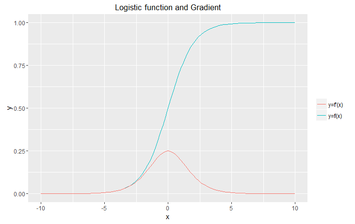

---

---

ggplot2 commands for plot

    # Define logistic fn and it's first derivative.
    f1 <- function(x) 1 / (exp(-x)+1)  
    f2 <- function(x) f1(x)*(1-f1(x))

    # import ggplot.
    library("ggplot2")

    # generate plot
    ggplot(data.frame(x = c(-10, 10)), aes(x)) + stat_function(fun = f1, aes(colour="y=f(x)"))+ stat_function(fun = f2, aes(colour="y=f'(x)")) + ggtitle("Logistic function and Gradient") + xlab("x") + ylab("y") + theme(legend.title=element_blank())
            

Colin,
December 4th, 2016

---