
Estimating a Biased Coin
Consider a coin with bias B, i.e. with probability B of landing heads up when we flip it:
\begin{align} P(H) &= B \\ P(T) &= 1-B \end{align}
We have a source of new coins (i.e. an infinite pile of coins), and each coin has a randomly assigned bias uniformly distributed over the interval [0,1].
NB. In practice we can achieve the full range of biases by bending coins, although the focus here is on the maths rather than the coin analogy.
Question 1
We take a coin from the pile and flip it once; what is the probability of flipping heads? (I.e. before we've observed any flips of the coin.)
Each coin we take from the pile has a defined bias B but we don't know what B is for each chosen coin, if we did we could say that P(H) = B for each known value of B. In the absence of knowing each specific B the probability of flipping heads is given by the expectation for B:
$$ P(H) = \Bbb E[B] = \frac{1}{2} $$
Expectation (Estimate)
Expectation is the value we expect to see on average, e.g. one way of defining `\Bbb E[B]` is as the result of averaging over an infinite number of samples. For less than infinity samples we get the estimate:
$$ \hat{\Bbb E}[B] = \frac{N_H}{N} $$
Noting that this estimate is poor for very small N; approaches the correct value with increasing N, and is exact for N=infinity:
$$ \lim \limits_{N \to \infty} \hat{\Bbb E}[B] = \Bbb E[B] $$
NB. We can explore this estimation method with a computer simulation that keeps a running update of the estimate `N_H/N` on an increasing number of samples (see Source code #1: Numerical analysis of a single coin flip)
By taking infinity samples we get a perfect reconstruction of B's uniform distribution, i.e. all possible outcomes are represented, each with their correct proportion within the full set of samples as defined by the uniform distribution over B.
Expectation (Exact)
We can obtain a closed form expression for the exact value of `\Bbb E[B]` by using B's probability density function directly, i.e. instead of recreating the distribution by taking infinity samples.
A uniform probability density function over interval [0,1] is given by:
$$ f(x) = \begin{cases} 1, & \text{for 0 <= x <= 1} \\ 0 & \text{otherwise} \\ \end{cases} $$
Multiplying by `x` gives an expression representing each possible sample value multiplied by its probability:
$$ x \cdot f(x) = \begin{cases} x, & \text{for 0 <= x <= 1} \\ 0 & \text{otherwise} \\ \end{cases} $$
Integrating (i.e. summing over the interval [0,1]) gives us our average, i.e. the expected value of B:
\begin{align} \Bbb E[B] &= \int _0^1 x \\[2ex] &= \left[\frac{x^2}{2} + C \right]_0^1 = \frac{1}{2}\\[2ex] \end{align}
Also see Question 1 Supplemental: Expectation of a uniform distribution with interval [a,b]
Question 2
We take a coin from the pile and flip it once. For those coins that flip heads what is the probability
of a second flip also being heads?
(I.e. what is our new estimate of B for those coins that have flipped heads once?)
We know that:
- B > 0, i.e. B cannot be exactly zero.
- B is unlikely to be a very small value, but it might be.
The probability of flipping two heads is given by:
$$ P(HH) = P(H) \cdot P(H) = B^2 $$
The probability of flipping one heads and one tails is given by:
$$ P(HT) = B (1-B) $$
Generalising, the probability of flipping a given sequence S consisting of `h` heads and `t` tails, for a given bias `B`, is:
$$ P(S|B) = B^h (1-B)^t \tag{1}$$
For a fixed S we can plot P(S|B) over the interval B=0 to 1, and this is in fact the Likelihood function for B, and is typically written with the two variables swapped, like so:
$$ \mathcal{L}(B|S) = P(S|B) $$
This reads as - the likelihood of B given S is equal to the probability of S given B. The likelihood notation emphasises that we have fixed S (the observed data), and that B is the variable being explored.
Since B is a probability its value is limited to the interval [0,1] and therefore for a given S we can plot our likelihood function over B's full range. There follows a series of such plots, one each for a different S (six example sets of observed outcomes).
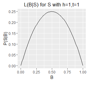


Likelihood functions for six different sets of observations.
Observations
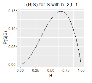
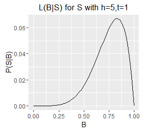
- Note the very different ranges on the Y axes; this corresponds with longer sequences (e.g. h=5,t=1) generally having a lower probability of occurring than shorter ones (e.g. h=1, t=0).
- The longer sequences also have spikier plots; this corresponds with our estimate of B becoming more well defined with an increasing number of observations (which are samples from B). Recall from question 1 that we can obtain an exact value for B by taking an infinite number of samples; each additional sample provides additional information about the true value of B, as such, as the number of samples increases some values of B become increasingly unlikely.
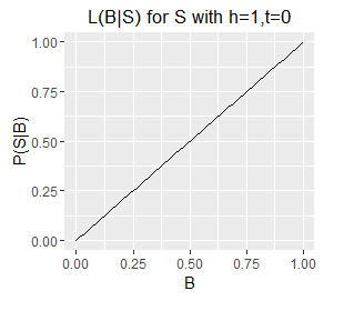
- Note also that the mode of each plot corresponds with the `B = h/N`, i.e. the proportion of samples that are heads. This holds even for a sample size of 1, where the likelihood describes a diagonal line with the mode located at B=0 or B=1 for a single T or a single H respectively. However, note that a single heads does not rule out a very low value of B, although low values of B are unlikely. The only claim we can make with certainty on observing a single H is that B does not equal exactly zero.
Integrating Likelihood (Discussion)
By summing the values of P(S|B) over the full range of B we marginalise B, i.e. we obtain a single value for P(S) given an unknown and uniformly distributed B, i.e.:
$$ P(S) = \int _0^1 P(S|B) dB \tag{2} $$
NB. If B was not uniformly distributed then P(S) may still be obtained by calculating a weighted sum over P(S|B), with weights defined by B's probability density function.
At this point it's worth considering the similarities and differences between our likelihood functions from figure 1, and a probability density function (PDF). A PDF can also be integrated to arrive at a single probability value, however, a PDF describes probability densities rather than probabilities, so how is it that we came to sum probabilities to arrive at a probability rather than summing probability densities?
The answer is that our likelihood functions describe both probability and probability density. This has come about because the free variable B is itself a probability and therefore bounded by the interval [0,1] (the 'unit length'). I.e. probability density is essentially normalised probability, or probability scaled per unit length; hence when the full range of the free variable is [0,1] then no scaling is required to convert a probability value to a probability density value.
Note however that although our likelihood functions describe probability density, they do not sum to 1 and therefore do not qualify as a PDF; this is merely a convention of terminology, since they are functions that describe probability density!
Likelihood Bounded by the Unit Square
As discussed above the free variable B is bounded by the interval [0,1], thus both the X and Y axes of our likelihood functions have interval [0,1] and our plots are bounded by the unit square. Therefore for one of our likelihood functions to sum to 1.0 (i.e. to achieve P(S)=1) each P(S|B) has to be 1.0, and for that to occur S would have to occur with certainty regardless of B, so effectively a process in which S always occurs and B has no influence.
Furthermore, our likelihood functions describe a dividing line in the unit square, with P(S) represented by the area below the line, and P(!S) the area above the line. The fact that we are dealing with unit squares is not of particular mathematical significance, but it does make for conveniently elegant plots. E.g. if we plot all six likelihood functions in the same unit square (i.e. at the same scale), then we see more clearly that the longer sequences are far less probable overall than the shorter ones, for any given B (single readings from the function), but also for unknown B (area under each curve).
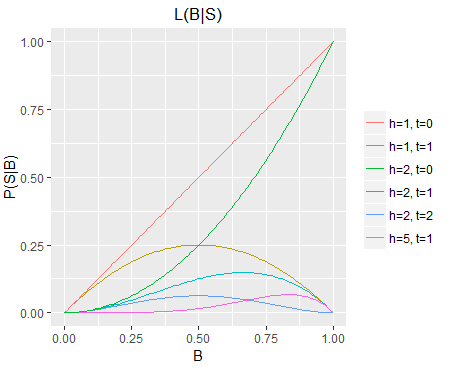
The six likelihood functions from figure 1
plotted at the same scale in a single unit square.
Alternate Solution to Question 1
The likelihood function for S with h=1, t=0 (the red diagonal) corresponds with the problem posed in question 1. Q1 effectively asked: what is P(H) given no observations and a uniformly distributed B? (noting that S=H in this case, and therefore P(S)=P(H)).
The likelihood function for h=1,t=0 represents the probability of flipping H for every possible value of B; integrating this function gives the total probability of P(H) given an unknown and uniformly distributed B. From the plot we can see visually that it is approximately one half, in agreement with the answer from question 1.
Integrating Likelihood (Derivation)
Restating (1), replacing B with x for clarity:
\begin{align} P(S|x) &= x^h (1-x)^t \tag{1} \\[1em] \int _0^1 P(S|x) dx &= \int _0^1 x^h (1-x)^t \\[1em] P(S) &= \int _0^1 x^h (1-x)^t &\text{applying (2)} \end{align}
We resolve the integral by restating in terms of the beta function. (NB. We can also resolve by repeated application of integration by parts.)
\begin{align} B(h,t) &= \int _0^1 x^{h-1} (1-x)^{t-1} dx \tag{beta function} \\[1em] &= \frac{(h-1)!(t-1)!}{(h+t-1)!} \end{align}
Giving:
\begin{align} P(S) &= B(h+1, t+1) \\[1em] P(S) &= \frac{h!t!}{(h+t+1)!} \tag{3} \end{align}
Expectation Given an Observed Sequence
The probability of flipping heads given an observed sequence S can be written as:
$$ P(SH | S) $$
I.e. the probability of a sequence consisting of S+H, given that we have already observed S. Applying Bayes' theorem:
$$ P(SH | S) = \frac{P(S|SH)P(SH)}{P(S)} $$
Note that P(S|SH) is always 1, i.e. if we've observed SH then S has already occurred; leaving:
$$ P(SH | S) = \frac{P(SH)}{P(S)}$$
Substituting in equation (3) to both the numerator and denominator:
\begin{align} P(SH | S) &= \frac{(h+1)!t!}{(h+t+2)!} \cdot \frac{(h+t+1)!}{h!t!} \\[1em] P(SH | S) &= \frac{h+1}{h+t+2} \tag{4} \end{align}
Noting that P(SH|S) is our expectation for B given S, hence we can also write (4) as:
$$ \Bbb E[B|S] = \frac{h+1}{h+t+2} $$
Concluding Question 2
If we observe a single H then h=1 and t=0; we can put these values into equation (4) to get:
$$ \Bbb E[B|H] = \frac{2}{3} $$
We can also explore and validate this relationship with a numerical analysis (see Source code #2: Numerical analysis of a single coin flip conditional on a single observed H)
Question 1 Supplemental: Expectation of a uniform distribution with interval [a,b]
A uniform probability density function over interval [a,b] is given by:
$$ f(x) = \begin{cases} \frac{1}{b-a}, & \text{for a <= x <= b} \\ 0 & \text{otherwise} \\ \end{cases} $$
Multiplying by `x` gives an expression representing each possible sample value multiplied by its probability:
$$ x \cdot f(x) = \begin{cases} \frac{x}{b-a}, & \text{for a <= x <= b} \\ 0 & \text{otherwise} \\ \end{cases}$$
Integrating (i.e. summing over the interval [a,b]) gives the expected value of samples from the distribution. Here `Z` represents a sample (or any sample, they all have the same expected value) from the p.d.f.
\begin{align} \Bbb E[Z] &= \int _a^b \frac{x}{b-a} dx \\[2ex] &= \frac{1}{b-a} \left[\frac{x^2}{2}\right]_a^b \\[2ex] &= \frac{1}{b-a} \left( \frac{b^2-a^2}{2} \right) \\[2ex] &= \frac{b^2-a^2}{2(b-a)} \\[2ex] \end{align}
Applying difference of squares, i.e: `b^2-a^2 = (b+a)(b-a)` :
\begin{align} \Bbb E[Z] &= \frac{(b+a)(b-a)}{2(b-a)} \\\\ &= \frac{b+a}{2} \\ \end{align}
E.g. for interval [0,1]; `a=0, b=1`, giving:
$$ \Bbb E[Z] = \frac{1}{2} $$
Source code #1: Numerical analysis of a single coin flip
    // C# Source
    private static void RunSimulation()
    {
        Random rng = new Random();
        int h = 0;
        int t = 0;
        for(;;)
        {
            for(int i=0; i<100_000_000; i++)
                                      {
                // Take a coin from the pile, i.e. sample B from a uniform random distribution.
                double b = rng.NextDouble();
                // Flip the coin once, with P(H) = b,
                // record the outcomes.
                if(rng.NextDouble() < b) { h++; } else { t++; }
            }
            // Report running estimates of P(H) and P(T)
            int total = h+t;
            double ph = (double)h/total;
            double pt = (double)t/total;
            Console.WriteLine($"P(h) {ph}, P(t) {pt}");
        }
    }
Source code #2: Numerical analysis of a single coin flip conditional on a single observed H
    // C# Source
    private static void RunSimulation()
    {
        Random rng = new Random();
        int h = 0;
        int t = 0;
        for(;;)
        {
            for(int i=0; i<100_000_000; i++)
                                      {
                // Take a coin from the pile, i.e. sample B from a uniform random distribution.
                double b = rng.NextDouble();
                // Flip the coin once, with P(H) = b.
                // If we flip heads then flip again and record the outcomes,
                // if we flip tails then just ignore and start again with another coin.
                if(rng.NextDouble() < b)
                {
                    // Heads; flip again.
                    if(rng.NextDouble() < b) { h++; } else { t++; }
                }
            }
            // Report running estimates of P(H) and P(T)
            int total = h+t;
            double ph = (double)h/total;
            double pt = (double)t/total;
            Console.WriteLine($"P(h) {ph}, P(t) {pt}");
        }
    }
ggplot2 commands for generating likelihood function plots
    # Define the six likelihood functions.
    f1 <- function(x) x^1 * (1-x)^1
    f2 <- function(x) x^2 * (1-x)^2
    f3 <- function(x) x^2 * (1-x)^1
    f4 <- function(x) x^5 * (1-x)^1
    f5 <- function(x) x^1 * (1-x)^0
    f6 <- function(x) x^2 * (1-x)^0

    # import ggplot.
    library("ggplot2")

    # Generate the six likelihood function plots.
    ggplot(data.frame(x = c(0, 1)), aes(x)) + stat_function(fun = f1) + ggtitle("L(B|S) for S with h=1,t=1") + xlab("B") + ylab("P(S|B)")
    ggplot(data.frame(x = c(0, 1)), aes(x)) + stat_function(fun = f2) + ggtitle("L(B|S) for S with h=2,t=2") + xlab("B") + ylab("P(S|B)")
    ggplot(data.frame(x = c(0, 1)), aes(x)) + stat_function(fun = f3) + ggtitle("L(B|S) for S with h=2,t=1") + xlab("B") + ylab("P(S|B)")
    ggplot(data.frame(x = c(0, 1)), aes(x)) + stat_function(fun = f4) + ggtitle("L(B|S) for S with h=5,t=1") + xlab("B") + ylab("P(S|B)")
    ggplot(data.frame(x = c(0, 1)), aes(x)) + stat_function(fun = f5) + ggtitle("L(B|S) for S with h=1,t=0") + xlab("B") + ylab("P(S|B)")
    ggplot(data.frame(x = c(0, 1)), aes(x)) + stat_function(fun = f6) + ggtitle("L(B|S) for S with h=2,t=0") + xlab("B") + ylab("P(S|B)")

    # Generate plot with all six likelihood functions.
    ggplot(data.frame(x = c(0, 1)), aes(x)) + stat_function(fun = f1, aes(colour="h=1, t=1"))+ stat_function(fun = f2, aes(colour="h=2, t=2")) + ggtitle("L(B|S)") + xlab("B") + ylab("P(S|B)") + theme(legend.title=element_blank())
Colin,
October 9th, 2016
 Copyright 2016 Colin
Green.
Copyright 2016 Colin
Green.
This article is licensed under a Creative Commons Attribution 3.0 License